Saddleback Large Thin Briefcase in Tobacco brown

I recently bought the Saddleback Large Thin Briefcase in the tobacco brown colour, and it arrived yesterday (2nd October 2013). The leather is amazing and it is an all around beautiful bag. The only problem is that it looks too big for my body size. I am 5'9 (178cm) and 150lb (70kg). Although I wanted the larger size to have the best fit for a 15" Macbook Pro I am just not tall/heavy enough for the large size to actually look good on me.

I am therefore trying to sell this beautiful bag. Currently it is listed on Gumtree.com.au at Saddleback Large Thin Briefcase - Tobacco

The briefcase has never been used, and is still in the original plastic wrapping. I have taken it out to have a look only. Saddleback briefcases are considered to be one of the best made leather briefcases on the market. With a 100 year warranty (even if you weren't the original purchaser) these are made to last. No zippers or snaps which will break, just high quality leather with double stitching and tough pigskin lining. These are the briefcases that will last you a lifetime. The leather is the best quality full grain leather, it looks and smells fantastic. The bags will look even better in a few years time, just have a look at some of the pictures online. Also comes with the free keychain that was included in the box. 

Exterior: 
16 ¾” W x 11 ½” H x 4 ½” D 
425mm W x 290mm H x 115mm D 

Interior: 
15 ¾” W x 11 ¾” H x 4” D 
400mm W x 300mm H x 100mm D 

A Review from Primer Magazine

The full product deatils are on the Saddleback Leather site.

Product Picture from Saddleback

Product Picture of interior from Saddleback

Front view

Side and back view

Back view

Front view with measuring tape for scale

Saddleback logo on the front strap

The first two photos are from the Saddleback website. About two days ago (30th Sept 2013) they updated the tobacco colour leather, so what you see on the website now is slightly different, although all the other details such as size are the same. The other pictures are of the actual bag. I will sell it for $450.

Can pick it up from me, or arrange to meet me somewhere and I can drop it off after work.

GPOPS - Optimisation Software

One of the major things missing from the CADAC4 software is the ability to calculate the optimum trajectory. This comes down to finding the optimal path given the known initial conditions (position and velocity) and the desired final conditions (orbital velocity and height). I have been doing a bit of reading of research papers dealing with this problem, however making the leap from the theory to the actual coding has been difficult. Mainly because I am not good enough at the maths to understand it properly.

Since it is unlikely that I will ever be able to code this myself, I did some more searching for an existing solution. I found the GPOPS software, which is a Matlab program for solving these sort of optimal control problems. Although there is still a lot to learn, one of the examples is a rocket launch with multiple stages. My aim is to learn this example and then create a clone of it with the DH-1 details. The input details will be determined by running CADAC4 and getting the velocity and position at stage separation. These will then be the inputs for the GPOPS run to determine the optimal path. It will be interesting to see how close the figures are to the book numbers! I will post some diagrams when I have gotten this done.

Running GPOPS

1. GPOPS can be downloaded from Sourceforge. I am running it under Matlab R2009b under Ubuntu.
2. Ensure that you have a large amount of swap space. I have had to increase mine to 16Gb.
3. Run the 'gpopsSetup' command from the unzipped directory.
4. Change to the 'examples/launch' directory and run 'launchMain' to start the run.

Developement Pathway to the DH-1

The two biggest barriers to getting the funding for building the DH-1 are:

1. The acceptance of simple engineering in the rocket area
2. Getting over he believability hump

Simple Engineering

The simple engineering approach is to cut back all the unnecessarily complex approaches to aerospace engineering and focus on building things that will work reliably. Accept the compromises where they need to be made instead getting bogged down trying to develope new technology to solve all the aspects of a problem. Focusing on the achievability of the whole mission, not any single piece of technology. An example of this is the design of the U2 spyplane with its unstable flight characteristics and unusual landing gear, but over the last 50  years it has proven to be one of the most effective ways of doing that high altitude spy missions. Being able to accept the compromises in design to achieve the mission is a big mental hurdle.

Instead of having the design drivers being low weight and maximum efficiency, have the design drivers as being the simplest approach which will enable to job to get done. This means that instead of trying to build the space shuttle, with its incredible complexity, we instead try to build a DC-3. Overengineering the first vehicle is not something to be avoided but encouraged! We simply dont know what the working environment will be for a reusable launch vehicle which operates on a daily or weekly basis. We therefore need to focus on getting a vehicle which will survive for a sufficiently long number of launches to prove the concept. The very first DH-1 will likely have a very small or zero payload. But it will truly be reusable, and the experience gained will be invaluable.

The Believability Hump

 The second barrier is the believabily hump. Most people will not be able to understand how simple and robust the DH-1 concept is until they see it in operation. Therefore we need to have a way of starting small while still keeping all the important aspects of the design. One idea which I have recently found is to first create a smaller reusable sounding rocket. This would be a single stage vehicle that combines both the first and second stage ideas. There is a very good article by Yoshifumi

Inatani over at www.spacefuture.com detailing the design of a reusable VTOVL design and the emphasis on reliable operability. Although it doesnt have the capability to reach orbital velocity it can still reach an altitude of over 300 km.

This rocket also has a payload of 100kg, which is a lot more than most sounding rockets, with a much larger payload bay volume as well! Because it is reusable with quick turnaround times it would greatly reduce the whole cycle of developing an experiment through to launching. I feel that if this cycle can be reduced to months instead of years then it will allow a lot more interesting work to be done. Instead of having a sounding rocket launch be a once in an education experience, it could be a once a semester type of experience. Most importantly it would show that the model of having much simpler yet more robust launch vehicles being turned around rapidly is a significant advantage.

I would envisage a small single stage reusable sounding rocket such as this being built for a couple of million dollars. The aim would be to assemble a small team of engineers to design and build this, operating on the X plane development model. This would enable the software and analysis to be done in smaller easier steps and verify the concept before too much money needs to be spent. This experience would then enable better engineering and design choices to be made once the full DH-1 developement occurs.

The Side Note

There is some great video footage from onboard the Armadillo Aerospace Stiga sounding rocket. An interesting look at what the world is like from 40km up!

Another talk which is interesting is by Kim Ennico (SETI), talking about Commercial Suborbital Spaceflight.

Running CADAC4 for the DH-1

This post is the documentation for running the CADAC4 program with the DH1 modules and inputs. All the software has been uploaded to a Google Code project called cadac4-dh1. The initial checkin was the version that I was running from my USB stick under windows,  using the gfortran compiler.

The second checkin was the code that I had under Linux, which can be compiled into an executable using the gfortran compiler.

To compile the main DH1 program, execute 'gfortran CADX3.FOR UTL3.FOR R3_MODULE.FOR'

The output will be an 'a.out' executable which should be renamed as 'DH1'. Running this program then reads the input files and calculates the TRAJ.ASC outputs. Refer to the CADAC4 documentation for full details.

Because I am not certain that compiling the Utility files is working correctly, I have also put the Windows/DOS versions of the utilities (CADIN3.exe etc) into a directory called DOS.

The output files can be plotted in Matlab. Start by opening Matlab in an X session:

/usr/local/Matlab/bin/matlab

First edit the TRAJ.ASC to remove all the headers and column names, t
hen change directory to the DH1 code, and execute the 'PlotGraph.m' script. This will generate a graph similar to the one shown.

 

The blue line is the altitude which tops out around 250,000 feet. The green lines and the right hand scale show the weight of the vehicle in kg, which starts off at 98,000kg GLOW.

PyDome Tutorial

Running PyDome

1.  Install Python. The code was developed under Python 2.7. Packages for all operating systems (Windows/Mac/Linux) are available from http://www.python.org/getit/ 
2. Create a directory under your users home directory and copy all the PyDome files there. This will be where you run the script from and save the output to.
3. Update the 'config.py' script to set the dome diameter and the geodesic frequency.
4. Run the 'geo.py' script from the command line. The default output is to print the results on the screen, so to save it to a text file just redirect the output:
   
   python geo.py > output.txt

An average desktop PC should take around 45 seconds to run for a 6V sphere, with lower frequency calculations taking even less time.

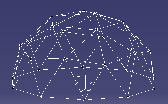
2V Dome results in CAD

Output

The output consists of the list of points with Cartesian coordinates:

/**********************************************************/

*     Points                                             *

/**********************************************************/

Pt77 = (-3782.10808464, 129.73646238, 4656.05271517)

Pt246 = (5547.56463791, 1201.67534466, 1944.35155109)

Pt112 = (4854.10196625, 3526.71151375, 0)

Pt402 = (1854.10196625, 4253.25404176, -3804.22606518)

Pt165 = (-571.430583503, -5647.38560167, -1944.35155109)

As well as the list of edges showing both endpoints and their coordinates:

/**********************************************************/

*     Edges                                              *

/**********************************************************/

Point Pt77 Edge List:

----------------------------------

Edge187: Pt74 = [ -3000.0, 974.759088699, 5103.90485011] - Pt77 = [ -3782.10808464, 129.73646238, 4656.05271517]

Edge188: Pt77 = [ -3782.10808464, 129.73646238, 4656.05271517] - Pt76 = [ -3917.72834195, 1272.94710279, 4362.45462008]

Edge200: Pt77 = [ -3782.10808464, 129.73646238, 4656.05271517] - Pt75 = [ -2736.75911987, -209.918005711, 5335.36165135]

Edge202: Pt83 = [ -3464.10161514, -1125.55484451, 4767.92683375] - Pt77 = [ -3782.10808464, 129.73646238, 4656.05271517]

Edge203: Pt79 = [ -4618.03398875, 449.02797658, 3804.22606518] - Pt77 = [ -3782.10808464, 129.73646238, 4656.05271517]

Edge204: Pt77 = [ -3782.10808464, 129.73646238, 4656.05271517] - Pt84 = [ -4428.16927497, -759.490479512, 3976.74377899]

Generated code for CAD Programs

It is easy to modify the code to generate output in a format which can be easily used in a CAD program. I have used CATIA for my examples, as it can run Visual Basic macros to do tasks. I simply created a macro which recorded the creation of two points and a line between them for an edge. Then I added the function ‘Get_CATIA_Desc’ to the Coordinates and Edges classes to print out the data with the right text. To generate all the points and edges in a CATIA part I just copy and paste this output into the VB editor and run the script.

Sample VB code to create a point in CATIA:

Set hybridShapePointCoord369 = hybridShapeFactory1.AddNewPointCoord(1958.86417097, -636.473551394, -5635.40172286)

body1.InsertHybridShape hybridShapePointCoord369

part1.InWorkObject = hybridShapePointCoord369

part1.Update

Program Structure

The advantage of using a language like Python is the Object Oriented (OO) nature of the language, which enables the code to reflect the structure. The objects which are modelled are the geodesic sphere (GeoSphere.py), icosahedron faces (IcoFace.py), edges, (Edge.py), and coordinates/points (Coordinates.py). The main GeoSphere class keeps track of a list of all the points and edges.

Algorithm

Each face of the icosahedron has known coordinates, as determined from the equations in Platonic Solids Tutorial. Given these coordinates we can process each of the 20 faces at a time and use vector maths to calculate the delta vectors from a starting point A to the other two corners B and C. The location of each of the intermediate points can then be determined by scaling the delta vectors according to the frequency, and then iterating to get each row and column. 

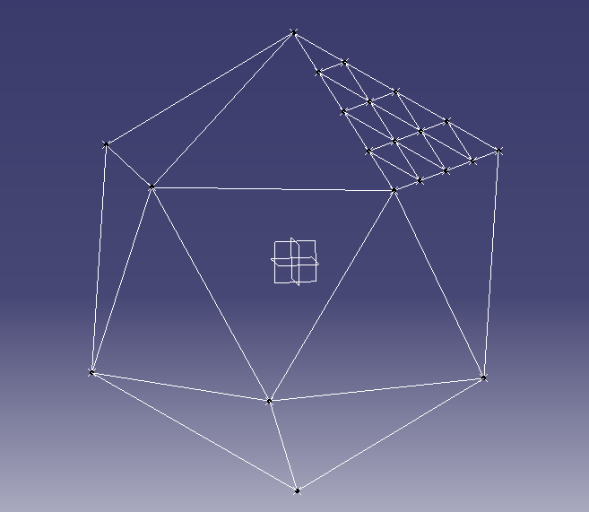
Icosahedron with one face divided for a 4V geodesic sphere

For example a frequency 4 dome would have each face divided into 4 rows and 4 columns.

The scaled delta vectors would then be calculated as: 

where f is the geodesic frequency.

With one counter for the row number and one for the column number, we can start at point A and use a loop over these counters to determine each point.

for i in range(0,self.freq_n+1): -- Row number

   for j in range( 1, self.freq_n - i + 1): -- Column number

                                                            

   # Calculate the new coordinates based on the offset from the initial point (A)

                                                               

As each face is added to the GeoDome class the coordinates from each face are added to the global list. Once all faces have been added then the list can be checked for duplicate points, as any points on the line where two faces meet will be doubled up.

The final step is to project each point onto the sphere. So far all the calculations have been in Cartesian coordinates (x,y,z), however the Coordinates class also keeps the polar coordinates (theta, phi, r). Each point will then have its polar coordinates radius (‘r’) set to the same value while keeping the angles theta and phi the same. Setting the radius will also recalculate the Cartesian coordinates for each point.

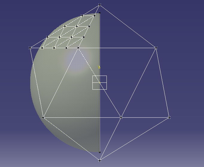
Icosahedron with sphere for projecting points

Advanced Modifications

 

The user parameters are defined in a small section at the beginning of the 'geo.py' script. Currently there are three parameters, the frequency of the geodesic (frequency_n), the radius of the dome (R_mm), and a flag for sphere or dome calculations. The coordinates should be entered in mm as this gives better readability in the final results.

To calculate the coordinates of a 6 metre (6000mm) radius dome of frequency 6, set these variables to the corresponding values as shown:

R_mm = 6000

frequency_n = 6
Dome_calc = True

There are potentially lots of different methods of dividing the faces of the icosahedron. Traditional geodesic domes or spheres divide each flat face into equal lengths. When the points are projected onto

the sphere they then have different lengths. An alternative method is to divide the arc between the edge vertices into equal angles. In order to change the calculation method for each face,

modify the file GeoSphere.py in the function Add_Face. This section of the code takes the 3 corner vertices and then calculates all the points within that face. Just replace the function 'Get_Edges_Equal_Distance'

with an equivalent function.

        #----------------------------------------------------

        # Use this function to divide faces by equal distance

        #

        edge_list = F1.Get_Edges_Equal_Distance()

To Do List

For each hub point calculate the angle of at which each edge meets at the hub. This would be both the angle between the edges and the angles of the edge from a flat plane.

Geodesic Domes using Python

Over the last few months I have been learning some of the maths behind geodesic domes. I was specifically interested in being able to generate the coordinates for all the points in a way which had enough accuracy to be able to use in a CAD program.

While I was investigating how the vertex points are generated I found this great site with all the information necessary to calculate the main points of the Icosahedron. From there the algorithm is fairly simple to explain, if a little harder to implement! Each of the 20 triangular faces is divided into smaller triangles according to the frequency of the dome. For example a 5V dome would have each face divided into 5 rows of equally sized triangles. From there each point is projected outwards onto a sphere to create the dome arrangement.

To make this easier and faster, I have written a small program in Python to do exactly this. At the moment it takes in the radius of the geodesic sphere and the frequency, and outputs the coordinates and edges. To make it easier I also made the printed output of the coordinates and edges as a piece of text which can be copied into the CATIA VB script tool, and then run as a VB script to automatically create the points and lines.

If you just want to print the cartesian coordinates then the printing of this CATIA code can be commented out.

As an example, here is a picture in CATIA of a frequency 9 dome with a 10 metre diameter.

Here is another one of a smaller frequency 5 sphere with a 4 metre diameter.

In order to share the code I have created a project on Google Code in a Subversion repository. You can download the code from PyDom or checkout directly with Subversion using the command:

svn checkout http://pydome.googlecode.com/svn/trunk/ pydome-read-only

Please let me know any suggestions for improvements!

The biggest enhancement to this script in the future will be the ability to calculate the angles at which the edges meet at each point. This would be crucial to enable the construction of the hubs to anchor all the edges.

Please let me know of any suggestions or fixes, keeping in mind that this is a work in progress!

Thanks,

Tim