PyDome Tutorial

Running PyDome

1.  Install Python. The code was developed under Python 2.7. Packages for all operating systems (Windows/Mac/Linux) are available from http://www.python.org/getit/ 
2. Create a directory under your users home directory and copy all the PyDome files there. This will be where you run the script from and save the output to.
3. Update the 'config.py' script to set the dome diameter and the geodesic frequency.
4. Run the 'geo.py' script from the command line. The default output is to print the results on the screen, so to save it to a text file just redirect the output:
   
   python geo.py > output.txt

An average desktop PC should take around 45 seconds to run for a 6V sphere, with lower frequency calculations taking even less time.

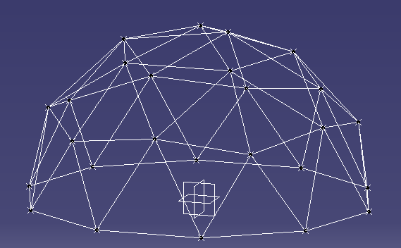
2V Dome results in CAD

Output

The output consists of the list of points with Cartesian coordinates:

/**********************************************************/

*     Points                                             *

/**********************************************************/

Pt77 = (-3782.10808464, 129.73646238, 4656.05271517)

Pt246 = (5547.56463791, 1201.67534466, 1944.35155109)

Pt112 = (4854.10196625, 3526.71151375, 0)

Pt402 = (1854.10196625, 4253.25404176, -3804.22606518)

Pt165 = (-571.430583503, -5647.38560167, -1944.35155109)

As well as the list of edges showing both endpoints and their coordinates:

/**********************************************************/

*     Edges                                              *

/**********************************************************/

Point Pt77 Edge List:

----------------------------------

Edge187: Pt74 = [ -3000.0, 974.759088699, 5103.90485011] - Pt77 = [ -3782.10808464, 129.73646238, 4656.05271517]

Edge188: Pt77 = [ -3782.10808464, 129.73646238, 4656.05271517] - Pt76 = [ -3917.72834195, 1272.94710279, 4362.45462008]

Edge200: Pt77 = [ -3782.10808464, 129.73646238, 4656.05271517] - Pt75 = [ -2736.75911987, -209.918005711, 5335.36165135]

Edge202: Pt83 = [ -3464.10161514, -1125.55484451, 4767.92683375] - Pt77 = [ -3782.10808464, 129.73646238, 4656.05271517]

Edge203: Pt79 = [ -4618.03398875, 449.02797658, 3804.22606518] - Pt77 = [ -3782.10808464, 129.73646238, 4656.05271517]

Edge204: Pt77 = [ -3782.10808464, 129.73646238, 4656.05271517] - Pt84 = [ -4428.16927497, -759.490479512, 3976.74377899]

Generated code for CAD Programs

It is easy to modify the code to generate output in a format which can be easily used in a CAD program. I have used CATIA for my examples, as it can run Visual Basic macros to do tasks. I simply created a macro which recorded the creation of two points and a line between them for an edge. Then I added the function ‘Get_CATIA_Desc’ to the Coordinates and Edges classes to print out the data with the right text. To generate all the points and edges in a CATIA part I just copy and paste this output into the VB editor and run the script.

Sample VB code to create a point in CATIA:

Set hybridShapePointCoord369 = hybridShapeFactory1.AddNewPointCoord(1958.86417097, -636.473551394, -5635.40172286)

body1.InsertHybridShape hybridShapePointCoord369

part1.InWorkObject = hybridShapePointCoord369

part1.Update

Program Structure

The advantage of using a language like Python is the Object Oriented (OO) nature of the language, which enables the code to reflect the structure. The objects which are modelled are the geodesic sphere (GeoSphere.py), icosahedron faces (IcoFace.py), edges, (Edge.py), and coordinates/points (Coordinates.py). The main GeoSphere class keeps track of a list of all the points and edges.

Algorithm

Each face of the icosahedron has known coordinates, as determined from the equations in Platonic Solids Tutorial. Given these coordinates we can process each of the 20 faces at a time and use vector maths to calculate the delta vectors from a starting point A to the other two corners B and C. The location of each of the intermediate points can then be determined by scaling the delta vectors according to the frequency, and then iterating to get each row and column. 

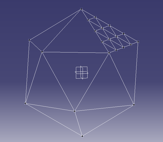
Icosahedron with one face divided for a 4V geodesic sphere

For example a frequency 4 dome would have each face divided into 4 rows and 4 columns.

The scaled delta vectors would then be calculated as: 

where f is the geodesic frequency.

With one counter for the row number and one for the column number, we can start at point A and use a loop over these counters to determine each point.

for i in range(0,self.freq_n+1): -- Row number

   for j in range( 1, self.freq_n - i + 1): -- Column number

                                                            

   # Calculate the new coordinates based on the offset from the initial point (A)

                                                               

As each face is added to the GeoDome class the coordinates from each face are added to the global list. Once all faces have been added then the list can be checked for duplicate points, as any points on the line where two faces meet will be doubled up.

The final step is to project each point onto the sphere. So far all the calculations have been in Cartesian coordinates (x,y,z), however the Coordinates class also keeps the polar coordinates (theta, phi, r). Each point will then have its polar coordinates radius (‘r’) set to the same value while keeping the angles theta and phi the same. Setting the radius will also recalculate the Cartesian coordinates for each point.

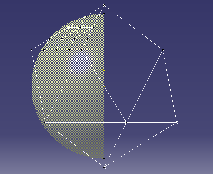
Icosahedron with sphere for projecting points

Advanced Modifications

 

The user parameters are defined in a small section at the beginning of the 'geo.py' script. Currently there are three parameters, the frequency of the geodesic (frequency_n), the radius of the dome (R_mm), and a flag for sphere or dome calculations. The coordinates should be entered in mm as this gives better readability in the final results.

To calculate the coordinates of a 6 metre (6000mm) radius dome of frequency 6, set these variables to the corresponding values as shown:

R_mm = 6000

frequency_n = 6
Dome_calc = True

There are potentially lots of different methods of dividing the faces of the icosahedron. Traditional geodesic domes or spheres divide each flat face into equal lengths. When the points are projected onto

the sphere they then have different lengths. An alternative method is to divide the arc between the edge vertices into equal angles. In order to change the calculation method for each face,

modify the file GeoSphere.py in the function Add_Face. This section of the code takes the 3 corner vertices and then calculates all the points within that face. Just replace the function 'Get_Edges_Equal_Distance'

with an equivalent function.

        #----------------------------------------------------

        # Use this function to divide faces by equal distance

        #

        edge_list = F1.Get_Edges_Equal_Distance()

To Do List

For each hub point calculate the angle of at which each edge meets at the hub. This would be both the angle between the edges and the angles of the edge from a flat plane.

Geodesic Domes using Python

Over the last few months I have been learning some of the maths behind geodesic domes. I was specifically interested in being able to generate the coordinates for all the points in a way which had enough accuracy to be able to use in a CAD program.

While I was investigating how the vertex points are generated I found this great site with all the information necessary to calculate the main points of the Icosahedron. From there the algorithm is fairly simple to explain, if a little harder to implement! Each of the 20 triangular faces is divided into smaller triangles according to the frequency of the dome. For example a 5V dome would have each face divided into 5 rows of equally sized triangles. From there each point is projected outwards onto a sphere to create the dome arrangement.

To make this easier and faster, I have written a small program in Python to do exactly this. At the moment it takes in the radius of the geodesic sphere and the frequency, and outputs the coordinates and edges. To make it easier I also made the printed output of the coordinates and edges as a piece of text which can be copied into the CATIA VB script tool, and then run as a VB script to automatically create the points and lines.

If you just want to print the cartesian coordinates then the printing of this CATIA code can be commented out.

As an example, here is a picture in CATIA of a frequency 9 dome with a 10 metre diameter.

Here is another one of a smaller frequency 5 sphere with a 4 metre diameter.

In order to share the code I have created a project on Google Code in a Subversion repository. You can download the code from PyDom or checkout directly with Subversion using the command:

svn checkout http://pydome.googlecode.com/svn/trunk/ pydome-read-only

Please let me know any suggestions for improvements!

The biggest enhancement to this script in the future will be the ability to calculate the angles at which the edges meet at each point. This would be crucial to enable the construction of the hubs to anchor all the edges.

Please let me know of any suggestions or fixes, keeping in mind that this is a work in progress!

Thanks,

Tim

DH-1 Dimensions

In preparation for making a CFD model in OpenFOAM, I have put together a drawing showing the main dimensions of the combined stage 1 and stage 2 vehicle. This gives me the data points to create a 2D model.

DH-1 Dimensions

CADAC Variable Locations

In the Fortran code for the CADAC4 software, variables are defined with a specific location. The number range is in the manual, however which variables are stored in which number location is not summarised. To help with this I wrote a Perl script to scan all the Fortran user modules and put together a list of all the names and locations. This helps me to know which spots are free for adding my own code, and means that if I do use a parameter it will have the same location.

CADAC4 Variable Locations

Updated Rocket Engine Data

I have been working on updating my summary of Rocket Engine Data. I have added in the Russian RD-192 engine, as it is about the right size for the main boost engine for the DH-1. I have been trying to find as much data on this as I can, because it runs on the Methane/LOX mixture which is of interest for the first stage.

I am also working on trying to get the OpenFOAM CFD software installed to try and get some basic numbers for the drag coefficients. At the moment the CADAC software is using the same coefficients from the basic sounding rocket example. Also the thrust calculation is a bit wrong because it assumes the exit pressure of the rocket will be the atmospheric pressure (Pe = Patm). However this is not the case especially for the sustainer RL-10A-4 engines.

Pictures of the DH-1

Using the dimensions specified in the book, I have put together a quick CAD model of what the DH-1 would look like. This is useful to get a feel for the size of the structure, and by putting a manikin into the scene it also gives an idea of the actual space inside as well. I will be working on this over time to improve it, but for now this is what I anticipate a fully reusable, two stage space launch vehicle to look like!

DH-1 Both stages. The porthole for 1st stage cabin is visible between the two jet engine pods

View from the rear. The 3 large purple objects are the main boost engines.

A closeup of the 2nd stage cabin area. The curved base of the heat shield, and the cutout for the boost motor are shown. The fuel tank for the second stage would be in this lower part of the structure.

Side profile of the first and second stages together. The manikin shows where the second stage cabin area would be between the two planes.

CADAC4 - Head.ASC

The two input files for the ROCKET.EXE executable are the HEAD.ASC and the CADIN.ASC. The HEAD file looks something like this:

 SCROLL NOECHOIN NOINTMSG NOSTGMSG NORANVAR NOTRAJBIN TRAJASC NOSTATBIN NOSTATASC NOTABOUT NOSWEEP
*
      51    REARTH       E Radius of the Earth = 6370987 - m
      52    CRAD         E Conversion factor = 57.29577951 (Deg/Rad)
      54    AGRAV        E Acceleration due to gravity @ sea level             =
      58    WEII3        E Earth Angular rotation = 7.2921154E-5 (rad/s)
     200    MAIR         D =0:Std Atmosphere, =1: Weather Deck
     201    TEMPK        G Atmospheric temperature - degK
     202    PRESS        O Atmospheric pressure - Pa
     203    RHO          O Atmospheric density - kg/m^3
     204    VSOUND       G Sonic speed - m/sec
 *   205    GRAV         O Gravity acceleration - m/s^2
     206    VMACH        O Mach number of rocket - ND
     207    PDYNMC       G Dynamic Pressure - Pa
    1200    MAERO        D =|MAERT|MAERV|, MAERT=1:Type, MAERV:Stage #
 *  1201    CD           O Drag coefficient - ND
 *  1202    CL           O Lift coefficient - ND
    1203    ALPHAX       D Angle of attack - deg
 *  1206    CA           G Axial force coefficient - ND

The original file is generated from the MKHEAD3.EXE program parsing the MODULE.FOR code and extracting all the parameters. However in order to get some output from the run, some of these parameters need to be marked as outputs. This is done by putting an asterisk ('*') in the second column. If there is no asterisk then this variable is not written to the TRAJ.ASC output file.